Continued fractions off�er a useful method and representation of expressing numbers and functions. One of interesting ideas of this method is that any number can be represented by a point on the real line and that falls between two integers.
Several attempts have been made during the last 100 years to develop continued fraction algorithm for complex numbers[1]; such algorithm having properties that are known to possess on the regular continued fraction algorithm in the real numbers case.
In the real case, for example, let  be any real number, and if
  is an integer, then
 .
.
There is one and only one such integer for any given real . The integer is sometimes called the floor of ,
![t= \left [ s \right ]](https://s0.wp.com/latex.php?latex=t%3D+%5Cleft+%5B+s+%5Cright+%5D&bg=ffffff&fg=000000&s=0&c=20201002)
For example : ![3= \left [ \pi \right ]](https://s0.wp.com/latex.php?latex=3%3D+%5Cleft+%5B+%5Cpi+%5Cright+%5D&bg=ffffff&fg=000000&s=0&c=20201002) ,
, ![-2= \left [-1.5 \right ]](https://s0.wp.com/latex.php?latex=-2%3D+%5Cleft+%5B-1.5+%5Cright+%5D&bg=ffffff&fg=000000&s=0&c=20201002) .
.
For any real with , there is a unique decomposition  where is an integer and
  is in the unit interval. So,
  if and only if
  is an integer.
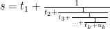
The process of finding the continued fraction expansion of a real number is a recursive process that procedes one step at a time. Given any real number , after  steps, the process goes like this one :
Which has integers  and real numbers
  that are members of the unit interval
  with
with  all positive. We can write another representation :
![s= \left [t_1,t_2,t_3,...,t_k+u_k \right]](https://s0.wp.com/latex.php?latex=s%3D+%5Cleft+%5Bt_1%2Ct_2%2Ct_3%2C...%2Ct_k%2Bu_k+%5Cright%5D&bg=ffffff&fg=000000&s=0&c=20201002) .
.
If  , the process ends after steps. Otherwise, the process continues at least one more step with
 .
.
In this way one associates with any real number a sequence, which could be either finite or infinite,  of integers. This sequence is called the continued fraction expansion of real number . For example,
  can be represented as a continued fraction

or ![\pi = \left [3, 7, 15, 1, 292, 1, 1, 1, 2, 1, 3 ...\right]](https://s0.wp.com/latex.php?latex=%5Cpi+%3D+%5Cleft+%5B3%2C+7%2C+15%2C+1%2C+292%2C+1%2C+1%2C+1%2C+2%2C+1%2C+3+...%5Cright%5D&bg=ffffff&fg=000000&s=0&c=20201002) .
.
Continued fractions have become more common in various other areas since the beginning of the twentieth century. For example, Robert M. Corless [2] examines the connection between theory of chaotic dynamical systems and continued fractions. It has also been used in computer algorithms for computing rational approximations to real numbers, as well as for solving Diophantine approximation of complex numbers [1] .
It turns out that complex numbers can also be represented as continued fractions, and, as such, falls between two Gaussian integers, and the unit is any divisor of  whose norm is 1.
The best method at the moment was devised by Asmus Schmidt. [1]
Let
![\mathbf{Z}\left [ i \right ] = \left\{a + bi : a, b \in \mathbf{Z},b \geq 0 \right\} \cup \left\{ \infty\right\}](https://s0.wp.com/latex.php?latex=%5Cmathbf%7BZ%7D%5Cleft+%5B+i+%5Cright+%5D+%3D+%5Cleft%5C%7Ba+%2B+bi+%3A+a%2C+b+%5Cin+%5Cmathbf%7BZ%7D%2Cb+%5Cgeq+0+%5Cright%5C%7D+%5Ccup+%5Cleft%5C%7B+%5Cinfty%5Cright%5C%7D&bg=ffffff&fg=000000&s=0&c=20201002) ,
,
![\mathbf{Z^{*}}\left [ i \right ]= \left \{ a+bi : a,b \in \mathbf{Z}, 0\leq a\leq 1, b\geq \left ( a-a^{2} \right )^{1/2} \right \}\cup \left \{ \infty \right \}](https://s0.wp.com/latex.php?latex=%5Cmathbf%7BZ%5E%7B%2A%7D%7D%5Cleft+%5B+i+%5Cright+%5D%3D+%5Cleft+%5C%7B+a%2Bbi+%3A+a%2Cb+%5Cin+%5Cmathbf%7BZ%7D%2C+0%5Cleq+a%5Cleq+1%2C+b%5Cgeq+%5Cleft+%28+a-a%5E%7B2%7D+%5Cright+%29%5E%7B1%2F2%7D+%5Cright+%5C%7D%5Ccup+%5Cleft+%5C%7B+%5Cinfty+%5Cright+%5C%7D&bg=ffffff&fg=000000&s=0&c=20201002) .
.
The set ![\mathbf{Z}[i] , \mathbf{Z}^{*}[i]](https://s0.wp.com/latex.php?latex=%5Cmathbf%7BZ%7D%5Bi%5D+%2C+%5Cmathbf%7BZ%7D%5E%7B%2A%7D%5Bi%5D&bg=ffffff&fg=000000&s=0&c=20201002) and their subdivisions into
and their subdivisions into
![\mathbf{Z}[i] = \mathbf{V_1}\cup \mathbf{V_2}\cup \mathbf{V_3}\cup \mathbf{E_1}\cup \mathbf{E_2}\cup \mathbf{E_3}\cup \mathbf{C},](https://s0.wp.com/latex.php?latex=%5Cmathbf%7BZ%7D%5Bi%5D+%3D+%5Cmathbf%7BV_1%7D%5Ccup+%5Cmathbf%7BV_2%7D%5Ccup+%5Cmathbf%7BV_3%7D%5Ccup+%5Cmathbf%7BE_1%7D%5Ccup+%5Cmathbf%7BE_2%7D%5Ccup+%5Cmathbf%7BE_3%7D%5Ccup+%5Cmathbf%7BC%7D%2C&bg=ffffff&fg=000000&s=0&c=20201002) and
and ![\mathbf{Z}^{*}[i] = \mathbf{V^{*}_1}\cup \mathbf{V^{*}_2}\cup \mathbf{V^{*}_3}\cup\mathbf{C^{*}}.](https://s0.wp.com/latex.php?latex=%5Cmathbf%7BZ%7D%5E%7B%2A%7D%5Bi%5D+%3D+%5Cmathbf%7BV%5E%7B%2A%7D_1%7D%5Ccup+%5Cmathbf%7BV%5E%7B%2A%7D_2%7D%5Ccup+%5Cmathbf%7BV%5E%7B%2A%7D_3%7D%5Ccup%5Cmathbf%7BC%5E%7B%2A%7D%7D.&bg=ffffff&fg=000000&s=0&c=20201002)
are shown in Fig. 1, Fig. 1*, respectively.
 Figure 1, Figure 1*. Every boundary point occurring in Fig. 1 is properly equivalent to a real number, and that every boundary point occurring in Fig. 1* is improperly equivalent to a real number. [1]
(Note : all regions are bounded by straight lines or circles with radii  (or part thereof), and are supposed to be closed;
  )
)
The 8 matrices  are defined as follows :

For any invertible matrix M,

with elements in  , let
, let  denote the corresponding homographic map :

And  denotes complex conjugation of .
A homographic map  is called unimodular if
 ![p,q,r,s\in \mathbf{Z}\left [ i \right ]](https://s0.wp.com/latex.php?latex=p%2Cq%2Cr%2Cs%5Cin+%5Cmathbf%7BZ%7D%5Cleft+%5B+i+%5Cright+%5D&bg=ffffff&fg=000000&s=0&c=20201002) (the ring of Gaussian integers) and
(the ring of Gaussian integers) and  . Notice that the determinant of a unimodular map is defined only as an element in the quotient group
  consisting of the two elements
  . A unimodular map is called properly unimoduIar if
  and improperly unimodular if
  .
.
An immediate consequence of these definitions is that every boundary point occurring in Fig. 1 is properly equivalent to a real number, and that every boundary point occurring in Fig. 1* is improperly equivalent to a real number.
A complex number, for example  can be represented as a series of these matrices:
  and so on. Multiplying them together would yield :

If the top and bottom are added up, the fraction  can be made, which approximately equals
  .
.  starts off
  .
.
The Asmus Schmidt method uses partitions to divide the complex plane into regions, then subregions, and so on, and in this way, each point is encoded by the sequence of regions to which it belongs. In the first generation :
 Figure 2. The first generation of Asmus Schmidt’s complex continued fraction method. (picture credite to Ed Pegg Jr., courtesy of MAA)
After that, each triangular region is divided into 4 parts, by adding a circle. In addition, each circle is divided into 8 regions, by adding 3 tangent circles.

Figure 3. The third generation of Asmus Schmidt’s complex continued fraction method. (picture credite to Ed Pegg Jr., courtesy of MAA)
Here is a portion of fourth generation :

Figure 4. The fourth generation of Asmus Schmidt’s complex continued fraction method. (picture credite to Ed Pegg Jr., courtesy of MAA)
Another interesting visualization on further successive generation was done by Mathematica software[7] in which seven matrices are used. Each use of these matrices divides the plane into seven parts as shown in the Figure 5.

Figure 5. Sucessive generations of Asmus Schmidt’s complex continued fraction method (picture credite to Doug Hensley, at Wolfram Library Archive).
References :
[1] Asmus L. Schmidt, Diophantine Approximation of Complex Numbers, University of Copenhagen, Denmark.
[2] Robert M. Corless, Continued Fractions and Chaos, Dept. Applied Math, University of Western Ontario, Canada.
[3] Ed Pegg Jr., Gaussian Numbers, editorial Math Games, March 15, 2004, MAA.
[4] MathWorld, Continued Fractions, Pi Continued Fraction.
[5] W. F. Hammond, Continued Fractions and the Euclidean Algorithm, Department of Mathematics and Statistics, University at Albany.
[6] Wikipedia, Continued Fraction, Generalized continued fraction, Gaussian integer.
[7] Wolfram Library Archive, Complex Continued Fractions, picture download : PDF document.


 ,
,  , and
, and  :
:")
 other viewpoints")
 Parametrization of Boy’s surface
 , so that giving the Cartesian coordinates
  of a point on the surface.


 ,
, varies from 0 to 1.
 di setiap langkah iterasi. Untuk itu diperlukan suatu ekspresi atau persamaan yang mengaitkan perubahan error
  di setiap layer, dimana nantinya didapat
  , seperti tampak pada gambar berikut :
 , bobot
  , dimana simbol
  …. (1)
 ….(2)
….(2) ….(3)
….(3)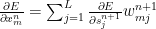 ….(4)
….(4) maka
maka ….(5)
….(5) ….(6)
….(6) bisa dinyatakan secara rekursif dengan melibatkan derivatif error terhadap output neuron pada layer berikutnya.
 Vesica Piscis, which literally means “the bladder of a fish” in Latin, becames the core of all solids. Image from
  Vesica Piscis with figures within. Image from
  , is not commensurable with its side. And this has given the area to be solved in other fashion, such as arithmetic or algebraic fashion. So that mathematics, particularly number theory, has been growing and developing with fascinating discoveries as we have seen today.
 Comic : Number line by


 ,
,  controls the girth.
 ,
,  , and
, and  :
:


 are usually called pseudospherical surfaces.
 is a surface with Gaussian curvature
  on
on  such that the first and second fundamental forms are:
 , and
, and  ,
, is the angle between asymptotic lines (the x-curves and t-curves). The


